Symplectic Basics III: The Cotangent Bundle

Now that we’ve gotten a little comfortable with the idea of a symplectic vector space, it shouldn’t take a huge leap of the imagination to say there’s a similar notion for (smooth) manifolds, too: they’re called symplectic manifolds (surprise). A (real, smooth) symplectic manifold of dimension $2n$ consists of a pair $(M,\omega)$ , where $M$ is the manifold, and $\omega$ is a closed, non-degenerate 2-form on $M$ (i.e., for all $p \in M$ , $\omega_p$ is an alternating bilinear form on the tangent space $T_p M$ , $d\omega = 0$ , and $\frac{1}{n!} \omega^n$ is a volume form on $M$ (equivalently, for all $p \in M$ , $\omega_p$ is a non-degenerate bilinear form on $T_pM$ ) ). In analogy with the case with symplectic vector spaces, $\omega$ picks out certain types of submanifolds of $M$ . That is, for a submanifold $N \subseteq (M,\omega)$ , we say $N$ is isotropic (resp., Lagrangian; resp., involutive) if, for all $p \in N$ , $T_p N \subseteq (T_pM, \omega_p)$ is an isotropic (resp., Lagrangian; resp., involutive) subspace. So, at face value, there doesn’t seem to be much of a change from the ordinary case of symplectic vector spaces, at least regarding these special types of submanifolds. Wrong, I was. I hope to talk about some of these things today.

Example 1. So, for baby’s first example of a symplectic manifold, we look at $M = \mathbb{R}^{2n}$ , equipped with the 2-form $\sigma_n \in \Omega^2(\mathbb{R}^{2n})$ (fyi, we write $\Omega^k(M)$ to denote the space of ( $C^\infty$ ) $k$ -forms on $M$ ) which has constant value $(\sigma_n)_p = \sigma_n$ on $T_p \mathbb{R}^{2n} \cong \mathbb{R}^{2n}$ , for all $p \in \mathbb{R}^{2n}$ . If you understood proposition 4 from my post about symplectic linear algebra (here: https://brainhelper.wordpress.com/2014/05/04/symplectic-basics/), you shouldn’t have any trouble with this example. The biggest change here is needing to work with differential forms on $\mathbb{R}^{2n}$ , not just a single bilinear form.

Let $(x;y) = (x_1,\cdots,x_n;y_1,\cdots,y_n) \in \mathbb{R}^{2n}$ be a (global) choice of linear coordinates on $\mathbb{R}^{2n}$ , and let $p = (x_0;y_0) \in \mathbb{R}^{2n}$ . Then,

$(\sigma_n)_p(v_1;v_2) := d_py \wedge d_px (v_1;v_2) = \sum_{i=1}^n (d_p y_i \wedge d_p x_i)(v_1;v_2)$

for $v_1,v_2 \in T_p \mathbb{R}^{2n} \cong \mathbb{R}^{2n}$ .

Example 2. As far as I’m (currently) concerned, these are the most important examples of symplectic manifolds: given any (real, smooth) manifold $M$ of dimension $n$ , the cotangent bundle $T^*M$ has a canonical symplectic structure. This is important, so I’ll go through most of the details on this one.

We’re going to need to conjure up some “canonical” symplectic form $\omega \in \Omega^2(T^*M)$ . There are essentially two ways to do this: first, a coordinate-free definition of $\omega$ ; after that, we’ll see what $\omega$ looks like in a system of coordinates to get a better feel for what we’re doing. The gist is that, on any cotangent bundle, we get a really useful 1-form for free, called the canonical 1-form (or tautological 1-form, or Liouville 1-form, or the Poincar\'{e} 1-form…), $\alpha \in \Omega^1(T^*M)$ .

Let $\pi : T^*M \to M$ be the projection map, $(x;\xi) \in T^*M$ (i.e., $x \in M$ is a point, and $\xi \in T_x^* M$ is a covector at $x$ ). Then, using the pullback $\pi^* : T^*M \to T^*(T^*M)$ , we define the value of $\alpha$ at $(x;\xi)$ to be

$\alpha_{(x;\xi)} := \pi_{(x;\xi)}^* (\xi)$ .

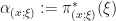This seems stranger/more abstruse than it actually is. From the definition of 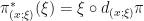$\pi_{(x;\xi)}^*$ , $\pi_{(x;\xi)}^*(\xi) = \xi \circ d_{(x;\xi)} \pi$ (this checks out: $\xi$ is, by definition, a linear map $T_xM \overset{\xi}{\to} \mathbb{R}$ , and $d_{(x;\xi)} \pi : T_{(x;\xi)}(T^*M) \to T_x M$ , so the composition at least makes sense). Finally, we define the “canonical” symplectic form $\omega$ on $T^*M$ to be $\omega := d\alpha$ (NB: some authors take $\omega = -d\alpha$ . It doesn’t really matter, since both choices give you a coordinate-independent construction of a symplectic form).

Now, suppose we have a local system of coordinates $(x) = (x_1,\cdots,x_n) \in M$ near $x_0$ , with associated linear coordinates 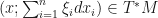$(x; \sum_{i=1}^n \xi_i dx_i) \in T^*M$ . What does $\alpha$ look like in these coordinates? Well, we know $\alpha_{(x;\xi)} := \pi_{(x;\xi)}^*( \xi)$ , so we just plug the coordinate expressions in and wind up with:

$\alpha= \pi^* (\sum_{i=1}^n \xi_i d x_i ) = \sum_{i=1}^n \xi_i d ( x_i \circ \pi) = \sum_{i=1}^n \xi_i dx_i$

(since $\pi(x;\xi) = x$ ). Hence, the canonical 1-form looks like $\alpha = \sum_{i=1}^n \xi_i dx_i$ in the local coordinates $(x;\xi)$ ; consequently, the symplectic form $\omega$ has the coordinate expression

$\omega = d\alpha = \sum_{i=1}^n d(\xi_i dx_i) = \sum_{i=1}^n d\xi_i \wedge dx_i$

near $x_0$ . In particular, since $\omega$ is exact, it is automatically a closed 2-form, and in these coordinates, it is easy to show that $\omega = d\alpha$ is non-degenerate, and that (had we started out with using coordinates, the above expression is independent of the coordinates chosen). The rest of the details are yours to check.

What’s the big deal? Why is $\alpha$ important/useful? Well, for one, it satisfies the following universal property:

proposition 1: The canonical 1-form $\alpha$ is uniquely characterized by the property that, for every 1-form $\eta : M \to T^*M$ (i.e., $\eta(x) = (x;\eta_x) \in T^*M$ is the graph of $\eta$ ), one has $\eta^* \alpha = \eta$ .

proof.

First, we note that $\eta^* : T^*(T^*M) \to T^*M$ , and

$\eta^* \alpha = \sum_{i=1}^n \eta^*(\xi_i dx_i) = \sum_{i=1}^n (\xi \circ \eta) d (x_i \circ \eta)$

$= \sum_{i=1}^n \eta_i dx_i = \eta$

is just the expression of $\eta$ in the local coordinates $(x; \sum_{i=1}^n \xi_i dx_i)$ on $T^*M$ . I’ll leave the proof of uniqueness of $\alpha$ to the reader 🙂

end proof.

Secondly, the canonical 1-form gives a really easy way to produce Lagrangian submanifolds of $(T^*M,\omega)$ . Let $\eta$ be a smooth 1-form on $M$ , and denote by $\Lambda_\eta := \{ (x;\eta_x) \in T^*M | x \in M\}$ the graph of $\eta$ . Then,

proposition 2: $\Lambda_\eta$ is a Lagrangian submanifold of $(T^*M,\omega)$ if and only if $\eta$ is closed.

proof:

Clearly, $\Lambda_\eta$ is a smooth submanifold of $T^*M$ of dimension $n$ (it’s diffeomorphic to $M$ itself). Then,

$\omega|_{\Lambda_\eta} = \eta^* \omega = \eta^* d\alpha = d(\eta^* \alpha) = d\eta$ ,

So $\omega$ vanishes on $\Lambda_\eta$ if and only if $d\eta = 0$ , i.e., if $\eta$ is closed.

end proof.

(Aside: for a symplectic vector space $(V,\sigma)$ (of dimension 2n), a basis $\{e_1,\cdots,e_n;f_1,\cdots, f_n\} \subset V$ is called a symplectic basis, provided $\sigma = \sum_{i=1}^n f_i^* \wedge e_i^*$ . In such case, we obtain the relations

$\sigma(e_i,e_j) = \sigma(f_i,f_j) = 0$ ,
$\sigma(e_i,f_j) = -\sigma(f_j,e_i) = -\delta_{ij}$ .

( $1 \leq i,j \leq n$ ). Additionally, in a symplectic basis, the Hamiltonian isomorphism $H : V^* \to V$ is given by

$H(e_j^* ) = -f_j$ .
$H(f_j^*) = e_j$ .

for $1\leq i \leq n$ (in the general case, $H : V^* \to V$ is defined by the formula $\langle \theta , v \rangle = \sigma(v,H(\theta))$ , where $\langle \bullet, \bullet \rangle : V^* \times V \to \mathbb{R}$ is the canonical pairing, and $\theta \in V^*, v \in V$ ). I forgot to talk about this in previous posts, and the Hamiltionian isomorphism has a really neat analogue for symplectic manifolds.

end aside.)

So, I’m giving you fair warning now: for the majority of examples/ situations I’ll talk about, the symplectic manifolds will always be of the form $(T^*M,\omega)$ for some smooth manifold $M$ . Okay. I was talking (secretively) about symplectic bases of symplectic vector spaces, and what the Hamiltonian isomorphism looks like when expressed in such a basis. For vector spaces, all we needed was for the (duals of) the basis elements to fit together in a regular way to form the original symplectic form (i.e., $\sigma = \sum_{i=1}^n f_i^* \wedge e_i^*$ ). But, for symplectic manifolds, the symplectic linear algebra takes place on the tangent space to every point; we don’t have the same freedom to choose “global” symplectic bases. The next best thing would be, of course, if we can at least always locally construct some analogue of symplectic bases, spanned by some frame of vector fields which would be a symplectic basis on each tangent space in a neighborhood of a point. Praise be upon us, for this is in fact the case: Darboux’s theorem guarantees that, for a smooth, 2n-dimensional symplectic manifold $(M,\omega)$ , for all $p \in M$ , there exists an open neighborhood $U$ of $p$ with smooth coordinate chart $(x_1,\cdots,x_n;y_1,\cdots,y_n) : U \overset{\thicksim}{\to} \mathbb{R}^{2n}$ (actually, this is a symplectomorphism as well!) such that $\omega_q = \sum_{j=1}^n d_q y_j \wedge d_q x_j$ for all $q \in U$ (one sometimes calls $(x;y)$ a system of Darboux coordinates, instead of/in addition to their symplectic properties). Luckily for us and our cotangent bundles, on $(T^*M,\omega)$ , any local system of cotangent coordinates $(x; \xi)$ on $T^*M$ serves as a system of Darboux coordinates, by our construction of $\omega$ . The most important thing to take away from Darboux’s theorem, however, is that all symplectic manifolds of a given dimension are (locally) the same! No distinguishing local invariants to be found here.

On $(T^*M, \omega)$ , the Hamiltonian isomorphism is the (fiber-wise) linear isomorphism $H : T^*(T^*M) \overset{\thicksim}{\to} T(T^*M)$ , and we’ll use it to construct some of the most important objects in symplectic geometry: Hamiltonian vector fields (check out Noether’s theorem, Hamiltonian dynamics, etc.). Precisely, given a smooth (real-valued) function $f$ on an open subset $U \subseteq T^*M$ , we define the Hamiltonian vector field of f, denoted by $H_f$ , to be the image of the differential $df$ under the Hamiltonian isomorphism $H : T^*(T^*M) \overset{\thicksim}{\to} T(T^*M)$ .

If we’ve chosen some local coordinates $(x;\xi)$ on $T^*M$ , our above discussion implies the vector field $H_f$ is given by

$H_f = \sum_{j=1}^n \frac{\partial f}{\partial \xi_j} \frac{\partial}{\partial x_j} - \frac{\partial f}{\partial x_j} \frac{\partial }{\partial \xi_j}$

Indeed, $\omega = \sum_{j=1}^n d \xi_j \wedge dx_j$ , so $H(dx_j ) = -\frac{\partial }{\partial \xi_j}$ , and $H(d\xi_j) = \frac{\partial}{\partial x_j}$ (for $1 \leq j \leq n$ ). Therefore,

$H_f := H(df) = \sum_{j=1}^n (\frac{\partial f}{\partial x_j}H(dx_j) + \frac{\partial f}{\partial \xi_j} H(d \xi_j) )$

from which result is immediate.

I really want to tie all this material together to talk about isotropic,Lagrangian, and involutive submanifolds of $(T^*M,\omega)$ , but I’ve already rambled on for quite a while in this post. If you’ve been following along these past few posts, you’ll remember that my original motivation for talking about these symplectic objects in $T^*M$ was for their relationship with the microsupport $SS(F)$ of sheaves in $D^b(M)$ . More precisely, for all $F \in D^b(M)$ , $SS(F) \subseteq T^*M$ is an involutive subset; if $F$ is also $\mathbb{R}$ -constructible, then $SS(F)$ is a Lagrangian subset of $T^*M$ . A little alarm should be going off in your head right now; there’s no reason at all for $SS(F)$ to be a smooth submanifold of $T^*M$ (take, for example, $F$ to be the constant sheaf supported on a singular subset of $M$ ), so how do these definitions apply? What details of the definition would we need to modify, and what changes? Let’s find out, next time.

References:

M. Kashiwara and P. Schapira, Sheaves on Manifolds (Appendix A).
A. Cannas de Silva, Lectures on Symplectic Geometry (http://www.math.ist.utl.pt/~acannas/Books/symplectic.pdf)
Alex Zamorzaev, notes from a course on introductory symplectic topology (http://math.stanford.edu/~alzaor/257a.html).

5 thoughts on “Symplectic Basics III: The Cotangent Bundle”

Joe Hannon says:

May 12, 2014 at 4:08 am

You didn’t go into the proof of Darboux at all, but I think it’s worth mentioning how it’s essentially a restatement of the $d\omega=0$ condition, which otherwise you have not justified (and has no analogue in linear algebra). Using Gram-Schmidt, you can orthonormalize a basis at a point, using a nondegenerate form (symmetric or alternative or neither), but in general cannot assume flat coordinates even in a tiny neighborhood of the point. There is a local geometric obstruction, curvature. Remove that obstruction and of course you have your flat (symplectic) coordinates.

Joe Hannon says:

May 12, 2014 at 4:09 am

Can you clarify what is the codomain of the Hamiltonian isomorphism? You’ve written it twice as cotangent vectors on the cotangent bundle?

1. Joe Hannon says:
  
  May 12, 2014 at 3:23 pm
  
  Ok, now the codomain of your Hamiltonian isomorphism is tangent vectors on the cotangent bundle. Can you also confirm the domain? You list it as cotangent vectors on the cotangent bundle. But then you write $H(df)$. $df$ is an element of the cotangent bundle, right? Not the cotangent of the cotangent?
  
  1. Joe Hannon says:
    
    May 12, 2014 at 6:26 pm
    
    I’m sorry, I misread it. Your function $f$ is a function on the cotangent bundle, not on the manifold. So $df$ is in the domain of $H$.
  2. brianhepler says:
    
    May 14, 2014 at 2:18 am
    
    Sorry, for some reason I didn’t get a notification of your comment. The Hamiltonian isomorphism sends covectors on $T^*M$ (elements of $T^*(T^*M)$ to vectors on $T^*M$ (now in $T(T^*M)$ ).
    
    I thought about doing the proof of Darboux’s theorem, and you present a valid point regarding justifying its existence at all. I suppose I’ve just been rushing to cover (and learn) these symplectic basics, so I can get a little more intuition for the involutivity of the microsupport (Lagrangian in the constructible case), and start to unravel Kashiwara and Schapira’s chapter on characteristic (and the sheaf of Lagrangian) cycles in $T^*M$ .